Face-Audio-Caption dataset, SOM of data, and LSTM-based lipreader
| Class | Instructor | Date | Language | Ta'ed | Code |
|---|---|---|---|---|---|
| CS 7476 Advanced Computer Vision | James Hays | Spring 2016 | MATLAB, Java | No | Code N/A |
| Class | Instructor | Date | Language | Ta'ed | Code |
|---|---|---|---|---|---|
| CS 7476 Advanced Computer Vision | James Hays | Spring 2016 | MATLAB, Java | No | Code N/A |
All the data we collected for our project can be found here (if unavailable, contact me via email): Dropbox repository of dataset.
All the code we used in our project can be found here : Githup repository of MATLAB and Java code.
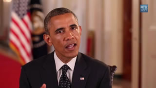
Figure 1. Screen Capture from a presidential address.
We present a dataset of aligned images, audio samples, and captions built from the President Obama's weekly addresses over the time period of 2009 to 2015, yielding a corpus of over 1.5 million image and audio samples and 205,000 conversationally spoken words. We also present the tools and methods we used to collect the data, with which a user can extract the same data from videos with provided closed caption files. Two pretrained 10,000 node Self-Organizing Maps are also included, one trained on half of the audio data samples and one trained on the mouth image samples, to be used to facilitate working with the high dimensional data. Lastly, we present an LSTM-based network trained on our dataset to associate sequences of mouth motions to captions (lip-reading) to demonstrate the set's utility.
There are many interesting problems in Computer Vision that depend upon more than a single image for a solution. Beyond the inherent complexities of recognition and classification commonly addressed in the field, with some tasks a single image doesn't present enough information, and instead sequences of images are necessary to even attempt to decipher the desired result.
One such problem is lip-reading, the recognition of spoken words through interpreting the motions of the speaker's face. This is difficult to accomplish using a purely instance-based classification mechanism, since, taking the english language for example, there are fewer unique mouth shapes a speaker will produce while speaking than there are unique units of sounds (called phonemes) that that speaker will be able to generate, rendering a one-to-one mapping between the two impossible.
These kinds of problems add another dimension, literally, to the already high dimensional problem space inherent in Computer Vision tasks, and require specialized algorithms that can learn sequential data, such as recurrent neural nets, to achieve useful results, along with specialized datasets by which these networks need to be trained. This is a challenge we hope to help address with our dataset.
We also present tools where similar data can be collected easily, as well as algorithms that can help the user analyze the collected data and use it in an efficient manner.
Lastly, we demonstrate our dataset on an LSTM-based network, where a subset of our data is used to train the network to assign captions to sequences of mouth motions. Similar lip-readers have recently come to prominence, and we demonstrate some of the particular strengths of our dataset with the results.
A quick survey of previous work reveals papers that have tried to solve the problem of lip reading using various well established methods that handle temporal data well. Previous work in this area has largely been focused on using probabilistic graphical models namely HMMs to model the lip movements. Matthws et al. [2] use HMMs to get about 44.6% accuracy on the task. ‘Eigenlips’ [3] used a hybrid approach of Multi-layered Perceptrons (MLP) and HMMs to get a good accuracy on a small dataset of around 2500 spoken letters. These methods were from the pre-deep learning era which did well only on a limited and constrained dataset. Potamianos et al. [1] mention that although progress on the audio-visual speech recognition has been made, but the systems are insufficient in performance for practical use.
Recently, a very interesting work related to this problem has been done by Ngiam et al. [4]. In their paper ‘Multimodal Deep Learning’, they employ layer-wise training with Restricted Boltzmann Machines (RBMs) followed by fine-tuning to learn features across an audio-visual training dataset. There is also work done by Hinton and Salakhutdinov to use deep learning to produce useful representations for handwritten digits and text.
The work that directly relates to our project is the one that came out recently titled 'Lip Reading with LSTM' [6] deals with the same problem. This work presents a plain vanilla LSTM with 2 layers to tackle the lip-reading problem using the GRID dataset from University of Sheffield. Although the accuracy achieved by this paper is about 79%, the GRID dataset is a corpus of limited words that covers fewer words than the dataset we created for this project. As we discuss later, the GRID corpus is also heavily curated and hence much cleaner and fitter for training a deep learning model. However, a model trained on the GRID dataset [13] may only have very limited success when applied to speech videos taken from a more realistic setting.
In order to create a system which could be applied to situations which are more realistic than ones in the GRID corpus, we set out to create our own dataset from existing youtube videos. Our final dataset consists of 1.5 million samples of face-cropped and isolated mouth images, and related audio samples. We also extract Frame-aligned mapping of the spoken words derived from closed caption files and audio analysis. The entire process of collecting these videos in their raw format and then converting them to a usable format for the LSTM is described in the next section. In this process we ended up creating a methodology and codebase to collect and process data from closed caption annotated videos. Another contribution is the creation of Self Organizing Maps trained on audio and image data.
We finally use the dataset we created in which we take the frame aligned mapping of words from videos and train them using an LSTM. The frames (which are cropped images) act as training samples with the words being the class. We experiment with a few variations of the LSTM architectures used to relatively great success in current LSTM lipreaders devising models that produced average (albeit unsatisfactory) results which we consider an important illustration in the utility of our dataset over existing similar datasets.
Our dataset differs from other similar datasets that we have found in numerous ways which we hope will serve to illustrate the utility we provide that was not previously available. Unlike many datasets, our set is of a single speaker, President Barrack Obama. While in many ways this could be perceived as a limitation, we hope that the fact that the data was collected over a period of 7 years, in multiple environments, serves to mitigate this somewhat. We also took some steps to help vary the data further, which we expand upon below.
One of the strengths of our dataset is its diversity. Over 8000 unique words are spoken over the course of our videos, over 3000 of which are spoken 5 or more times (which would yield at least 10 training examples using horizontal-axis mirroring of the face images). These words are spoken in a conversational manner, with sentences of varying cadence, and often indistinct boundaries between words, providing a more natural setting than a dataset built with the intention of training, for example, an Isolated Word Speech Recognizer.
Another strength of our dataset is in the source material itself. The videos we used to collect the data is high definition with clear audio, so the quality of the individual image frames and audio samples is very high. On the other hand, there is a natural variance built into the data since each weekly address source video was recorded one at a time, over the span of 7 years. The lighting and ambient sound, while consistent within a particular video, vary from video to video in a manner that is we have not seen in similar datasets - often the president is giving his speech in an outdoor location with very different lighting, or in a loud environment like a manufacturing plant, all of which serves to vary the resultant data in a useful manner and counter the limitation of having only one speaker.
Lastly, the videos have clear and accurate captions provided that, when combined with other processing driven by the audio samples, serve to indicate reasonable estimates of frame boundaries for individual words. These can be verified via synchronization with the audio samples, and also can be fine tuned with speech recognition.
All of the code required to process the source material and construct our dataset is included, except where otherwise specified (i.e. openFace for the face cropping transformations). We implemented the majority of our scripts in MATLAB, except for the caption-to-frame mapping code which is an Eclipse Java project.
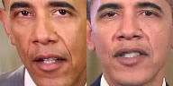
Figure 2. Two isolated face image samples, the left image using the outer eyes and nose as fixed points, the right using the inner eyes and bottom lip, of the same spoken word from two different videos.
To build our dataset we acquired 310 videos of President Obama giving weekly State of the Union addresses, over the period of time from 2009 to 2015, which amounted to over 30 hours of video. We sampled these videos to get individual frame images and the associated audio samples of what the president was saying, using the encoded sampling rate of the video itself, to preserve image alignment and help with caption alignment. The videos were originally recorded at either 25 or 30 frames per second. We then transformed and face-cropped the resultant images using the openFace library. To accomplish this we chose two sets of different desired fixed points on the faces (the outside points of the eyes and the nose, and the inside points of the eyes and the lower lip) which were then used to provide a basis to transform the face image as the speaker's head moved around while speaking. We used each set of fixed points on half of the image data, in an effort to help expand the diversity of the samples otherwise limited by the fact that they are generated by the same speaker, since each set of fixed points gives different mouth image results for the same word, as is seen in Figure 2. Each cropped face image in our dataset is 96 x 96 pixels of RGB data, and we also provide 40 x 40 gray scale images of the isolated mouth.
%Closed Caption Example
    %This is an example of the .vtt file for a passage of spoken
    %words from a video, including when these words are to be displayed.
    %(hr:min:sec:ms) --> (hr:min:sec:ms)

		00:01:11.400 --> 00:01:13.900
		Now we have to build
		on this progress.

		00:01:13.900 --> 00:01:16.667
		Congress should give every
		American the chance to refinance

		00:01:16.667 --> 00:01:19.100
		at today's low rates.

		00:01:19.100 --> 00:01:20.967
		We should help more qualified
		families get a mortgage

		00:01:20.967 --> 00:01:23.166
		and buy their first home.
Each source video included full transcriptions of the president's speech given in the .vtt closed caption format, which includes the time stamp offset from the beginning of the video determining when a set of words is to be displayed, as shown above. Using the assumption that the captions are displayed very close to when the words are spoken, which is a reasonable assumption since these videos are not live and are therefore not generating the captions via speech recognition, we developed an algorithm to estimate the frame bounds of each word, to be used to build associations between sequences of sound samples and words (for speech recognition training) or face/mouth images and words (for lipreader training).
First we had to convert all numeric and symbolic data to words, using the appropriate grammar depending on estimated context and inferred intent. For example, "17.76" would be translated as "seventeen point seven six" while "$17.76" would be translated as "seventeen dollars and seventy six cents"; "1776" would be "seventeen seventy six" and "$1.776 billion" would be translated as "one point seven seven six billion dollars" and "1,776" would be translated as "one thousand seven hundred and seventy six". This also came into play with website urls - "www.whitehouse.gov" would be translated as "double u double u double u dot whitehouse dot gov".
We would derive a frame boundary estimate for each word by assigning it a portion of the duration it would be displayed proportional to the word's letter-length footprint in the caption itself, including spaces. So given a caption displayed for 20 frames, starting at frame 100, consisting of the words "My Fellow Americans", we would estimate that "My" would display for 3 frames (100-103), "Fellow" would display for 7 frames (104-110), and "Americans would display for 10 (111-120).
We augmented this estimate by analyzing the audio data. By taking the RMS power of each frame's sample audio, we searched for values below a certain threshold and used them as suggestions of word breaks, as is shown in Figure 3. We chose the threshold so that we would find more word breaks than there were words spoken in the video to be sure we would find all of them.
Taking these suggestions we would then find the nearest audio-derived word breaks to each audio frame break suggested by the caption data and adjust the caption-derived break accordingly, with the caveat that any audio suggestion beyond a certain threshold would be ignored. A clip of an example of the bounds for some words yielded by our results can be found here : Example Of Isolated Words While this method was generally very successful in our random sampling and manual checking of the audio synchronization (with which we covered about 10% of the entire corpus), particularly with larger words, we realized that with smaller words the small window was often inaccurate by a few frames, as is evidenced in the video linked above, due to cadence variation or just inaccurate assumptions. When building our training data for the LSTM-based lipreader network, this discrepancy was mitigated somewhat by the mechanism we used to build the fixed-length sequence windows upon which we trained the network, as is discussed in relation to building our training data in Section 5.2.
Self Organizing Maps are networks of perceptrons where each node has a weight corresponding to a feature of the training data, which are initially randomly weighted. A training example is then mapped to the node whose weights most closely match its own feature values, and all the surrounding nodes within the current neighborhood (which decays in size over time) are modified to "look" more like the mapped node. Then, another example is mapped to a node, and the process is repeated. Once the entire batch of training examples is mapped, the neighborhood of impact decays and the mapping process is repeated with the now smaller neighborhood.
A SOM will yield a reasonable low-dimensional representation of high dimensional data, and is often used to visualize high dimensional data or as a dimensionality reduction mechanism where high dimensional data might have a low number of principal components. It can be used as a clustering algorithm in that it naturally maps similar examples to nearby nodes, without any required a-priori knowledge or choice of cluster size. The nature of how it is trained preserves a continuous topology among each weight/feature [4.4.1], enabling data-point generation through interpolation of node weights.
We chose to build SOMs on our audio and image data to not only reduce their dimension but also to potentially be used to generate data examples. For example, since the images of the various mouth configurations recorded are synchronized with each audio sample, we have a natural mapping from the SOM of visual mouth mappings to the SOM of audio samples generated. An input image of a mouth shape could then be mapped to a location on the image SOM, and the nearest surrounding nodes could then be used to provide interpolants of their corresponding nodes in the Audio Data SOM, yielding an audio sample result.
Our SOM implementation was achieved using the SOMOCLU library which is optimized for both openMPI-based cluster and GPU-based computing. We built a 10,000 node SOM for both the audio data and the image data, and trained both of them on the first 90 videos worth of our image dataset. While no sequence data was recorded in the mappings, limiting their usefulness for sequence learning, the decrease in dimensionality of the data, particularly for the images, implies the potential of longer training sequences while negatively impacting the training time, and experiments using this representation of our data in this capacity are ongoing. Both SOM maps are provided along with our dataset repository.
The use of Recurrent Networks to allow a sequence of input vectors to be considered at any given time for training. ConvNets suffer from a huge limitation in that they operate over a fixed input size and produce a fixed sized output in return and don't have the ability to work on sequence of input vectors. This makes RNNs the default network architectures in the neural network world to try and model inputs that have a temporal aspect to them. The case of lip reading too requires us to work on a sequence on input frames and have the model predict an output class.
LSTMs have worked very well in the recent past on problems that involve sequential inputs such as speech recognition [9]. LSTMs are a much more powerful version of RNNs due to their ability to overcome the vanishing gradient problem which allows significant events to affect the hidden weights of the network over a longer sequence of inputs [10]. LSTMs are useful in this context because we are looking at sequence length that typical RNNs do not have the capability to handle. Given the larger memory of LSTMs, it is more useful for our use case.
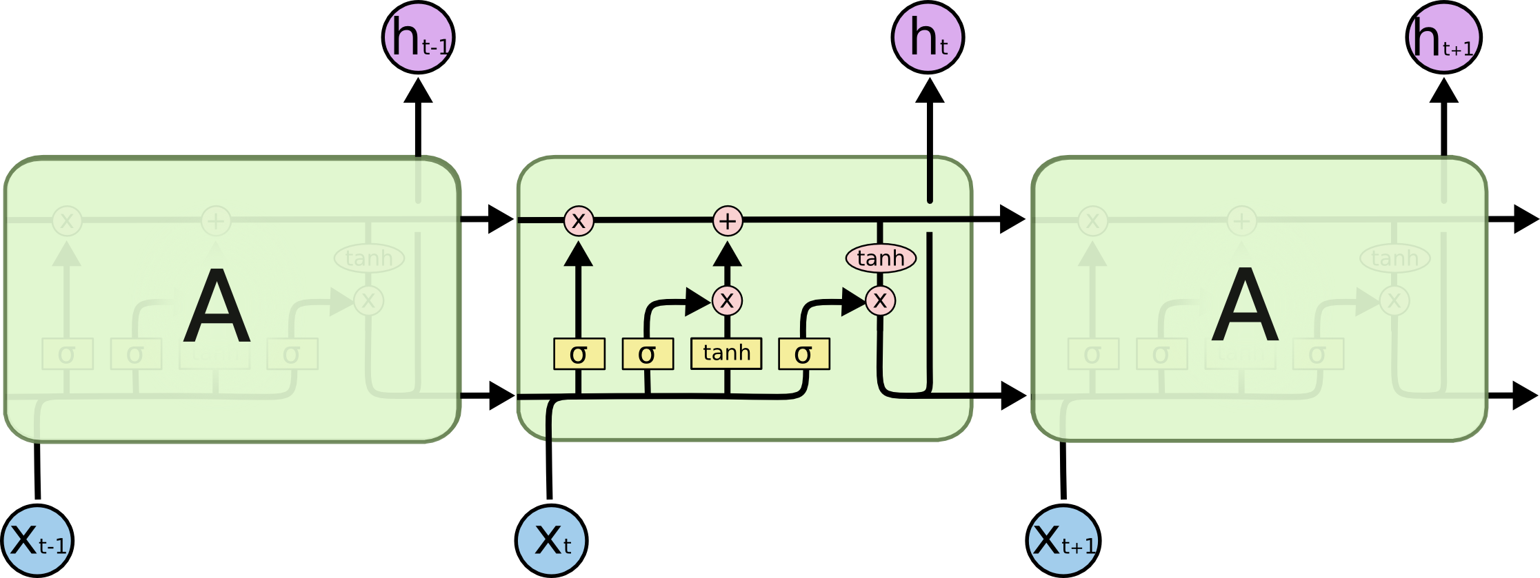
Fig: Repeating LSTM modules
What's different in the LSTM (as shown in the figure above) is the presence of memory cells which allow inputs events in longer sequences to be held in the 'memory'. The cell state from these memory cells affects the way in which the hidden units of the LSTM are updated. These memory units have what are called 'gates' which can control the flow of gradients and can also allow for operation such as resetting the memory as and when required.
For the training data we used in to train the LSTM lipreader, we chose a subset of our word data consisting of 33 words of high frequency of occurance (at least 300 occurances each). We isolated the image frames of each occurance in 3-dimensional MATLAB matrices where each column was an image of the cropped grayscale mouth (1600 pixels), each row denoted a particular pixel in this image, and each page denoted a particular training example. We built a similar 3-dimensional matrix for our labels, where each word was represented by a 1-hot vector corresponding to the sequence being classified. This process was automated, and the code to do this is included, so that all that is required is a csv file of the desired words fed to the java program that also generates caption frame estimates. The resultant file "training_DataNumericDict.csv" is then used by the MATLAB script "testTrainingDataLoad.m" to generate the training data.
Since we used a fixed sequence length across all words, we had to pad or truncate our training data based on the length of a particular word in samples compared to our chosen sequence length, which was 25 frames. To process each word, first we aligned the word's frames to be centered in the sequence map. Then, if the word was too long, we clipped frames from the edges, favoring ending frames for an odd number of overflow frames.
If the word was shorter than the sequence, we would add extra frames sufficient to cover half of the existing margin, and then fill the rest of the space with empty frames. So, for example, if a word was 5 frames long, we would add 5 frames of source material both before and after the word, and then add the rest as silence. This also helped with mis-alignment with very small words, since given the sequence length of 25 frames (approximately a second) we held great confidence that even our imperfect frame estimates would be sufficient coupled with this buffer of source material (which was larger for the smaller words most likely to be misaligned) to find the word in the source material.
The LSTM implementation we use in our project is a vectorized matlab implementation of LSTM which was created by researchers from the University of Hong Kong[11]. They created this to solve the problem of trying to identify the speaker who is talking at any given time in a video [12]. The vectorized LSTM or vLSTM is implemented in matlab with support for CUDA enabled GPUs for optimization.
Our implementation uses a vanilla LSTM model with any modifications to the input, forget or output gates of the LSTM. We experimented with both 1 and 2 layered LSTM. In a two layered LSTM, the output from the hidden layer of the first LSTM goes directly as the input to the hidden layer of the second LSTM. As mentioned above, our input sequence length to the LSTM was 25 and we had a batch size of 50. The batch size indicated the number of training sequences being fed to the LSTM as input. The input per sequence was 25 vectors with 1600 dimensions (since we only used grayscale image crops). For the single layer LSTM, we used a hidden size of 512 units and for the 2 layer LSTM, the hidden units' size at each level was 256.
The results we saw when training the models on our dataset, while substantially better than random, were not as good as similar results seen by similarly constructed models, such as those reported in [6]. This could be attributed to the noisy nature of our training data, which is by design. As mentioned earleir, we do not present a dataset of isolated individual words, such as the GRID corpus [13] used by [6], but rather words being used in conversational speaking.
This rather un-curated nature of our dataset does make it difficult for us to train reliably due to the high level of noise in the data. In the model that we ran, we performed a 33-way classification where each class corresponded to a word. Our results varied between 25% - 30% for a 2 layer LSTM model which was run for about 200 epochs. The single layer LSTM model performed worse with about 20% accuracy. Random chance for this problem is at 3%. Unfortunately after running for about 200 epochs we did not see any convergence between the training and the testing curves. Once reason for this, we think, is that there is a poor correspondence between the order in which the classes are encountered by the model from the training and the test batches.
For future work, there are numerous expansions to our dataset we would like to implement to more accurately present the data we have, as well as to expand our corpus.
One component we would like to implement would be a speech recognition engine to more cleanly specify frame-based word boundaries in the image/audio data. While our estimation method worked well, it was not perfect, and a well trained speech recognizer would undoubtedly be able to quickly isolate the appropriate frames for each word in the corpus. This task is made even easier given our word suggestions and frame estimations.
Another desirable expansion would be augmenting the dataset with more speakers. Many news programs and talkshows are available on youtube where an individual speaker is featured, face isolated and professionally recorded. Using the collection methods and code we have accumulated it would not be difficult to process these clips in a similar manner and expand the dataset to cover other speakers.
The nature of the SOM-based models and their potential as generative tools is intriguing. It would be interesting to explore the extent by which a SOM representation of the data can embed the essential nature of the source material required for successful sequence learning, which could prove a promising mechanism to more quickly and efficiently train algorithms on sequences.
[1] Potamianos, G., Neti, C., Gravier, G., Garg, A., & Senior, A. W. (2003). Recent advances in the automatic recognition of audiovisual speech. Proceedings of the IEEE, 91(9), 1306-1326.
[2] Matthews, I., Cootes, T. F., Bangham, J. A., Cox, S., & Harvey, R. (2002). Extraction of visual features for lip-reading. Pattern Analysis and Machine Intelligence, IEEE Transactions on, 24(2), 198-213.
[3] Bregler, C., & Konig, Y. (1994, April). “Eigenlips” for robust speech recognition. In Acoustics, Speech, and Signal Processing, 1994. ICASSP-94., 1994 IEEE International Conference on (Vol. 2, pp. II-669). IEEE.
[4] Ngiam, J., Khosla, A., Kim, M., Nam, J., Lee, H., & Ng, A. Y. (2011). Multimodal deep learning. In Proceedings of the 28th international conference on machine learning (ICML-11) (pp. 689-696).
[5] Graves, Alex; Mohamed, Abdel-rahman; Hinton, Geoffrey (2013). "Speech Recognition with Deep Recurrent Neural Networks". Acoustics, Speech and Signal Processing (ICASSP), 2013 IEEE International Conference on: 6645–6649.
[6] "Lipreading with Long Short-Term Memory", by Michael Wand, Jan Koutnik, Jurgen Schmidhuber, 2016
[7] "Learning from Data: Concepts, Theory, and Methods", by Vladimir Cherkassky, Filip M. Mulier
[8] “An Audio-Visual Corpus for Speech Perception and Automatic Speech Recognition,” M. Cooke, J. Barker, S. Cunningham, and X. Shao, 2006
[9] Graves, Alan, Abdel-rahman Mohamed, and Geoffrey Hinton. "Speech recognition with deep recurrent neural networks." Acoustics, Speech and Signal Processing (ICASSP), 2013 IEEE International Conference on. IEEE, 2013.
[10] Graves, Alex, and Jürgen Schmidhuber. "Framewise phoneme classification with bidirectional LSTM and other neural network architectures." Neural Networks 18.5 (2005): 602-610.
[11] https://github.com/jimmy-ren/lstm_speaker_naming_aaai16
[12] Ren, Jimmy, et al. "Look, Listen and Learn-A Multimodal LSTM for Speaker Identification." arXiv preprint arXiv:1602.04364 (2016).
[13] Cooke, Martin, et al. "An audio-visual corpus for speech perception and automatic speech recognition." The Journal of the Acoustical Society of America 120.5 (2006): 2421-2424.
Copyright © 2015 - All Rights Reserved - johnmturner.com
Template by OS Templates